Back to the lesson·Lesson 5 of 8·Judging a survey
Can this survey be believed?
The same deck as the downloads, rendered as a page. Start the slideshow to present it full screen — arrow keys or a click advance one slide, Escape leaves.
What this lesson covers
- A survey is accepted or it is not
- The checks
- Flags
- The standard deviation
- Digit preference
- Age heaping
- Sex ratio and team bias
- The verdict
- Write it up without accusing anyone
- What comes next
Speaker notes
The SMART plausibility report, on a survey that fails two of its checks. A standard deviation of 1.22, one team measuring 0.6 z-scores low, 69% of its heights on a half centimetre, and a quarter of ages on a whole year.A survey is accepted or it is not
- The SMART methodology does something unusual and valuable: it publishes a set of checks a survey must pass before its prevalence is used, and the checks are computable from the survey's own data.
Speaker notes
The SMART methodology does something unusual and valuable: it publishes a set of checks a survey must pass before its prevalence is used, and the checks are computable from the survey's own data. That means a survey can be rejected on its own evidence, before any argument about what the number means. This lesson runs the checks on the platform's SMART survey, which passes some and fails others.The checks
Check What it detects Acceptable Flagged records Impossible or extreme measurements under about 2.5% Standard deviation of WHZ Measurement error inflating the spread 0.8 to 1.2 Digit preference Rounding rather than reading low, and even across teams Age heaping Age estimated rather than documented low Sex ratio Selection bias in who was measured near 1.0 Team bias One team measuring differently means close across teams Flags — In Python
computable = smart["whz"].notna() flagged = computable & ~smart["whz"].between(-5, 5) print(f"{computable.sum()} computable, {flagged.sum()} flagged " f"({flagged.sum() / computable.sum():.1%})")Flags — In R
smart |>
  filter(!is.na(whz)) |>
  summarise(n = n(), flagged = sum(!between(whz, -5, 5)),
            rate = flagged / n)
Speaker notes
12 of 864, about 1.4%. Passes. A flag rate above a few percent means measurement or entry problems severe enough to question everything else, so this check runs first and gates the rest.The standard deviation — In Python
analysable = smart.loc[smart["whz"].between(-5, 5), "whz"] print(f"n = {len(analysable)}, mean = {analysable.mean():.2f}, " f"sd = {analysable.std():.2f}")The standard deviation — In R
smart |> filter(between(whz, -5, 5)) |> summarise(n = n(), sd = sd(whz))The standard deviation
- 1.22 — Outside the acceptable band, at the top edge
- Measurement error. Random error in weight or height widens the distribution without changing its centre. The…
- A genuinely heterogeneous population. Two very different sub-populations sampled together.
- Entry error. Transposed digits, wrong units, mixed-up records.
- An inflated SD raises the prevalence — A wider distribution puts more children past a fixed cut-off, so GAM rises…
Speaker notes
1.22. Outside the acceptable band, at the top edge. This is the most important number in a plausibility report and it is worth being precise about why. The WHO reference population has a standard deviation of 1 by construction. A real population is slightly more variable, so 1.0 to 1.2 is what a well-measured survey produces. Above that, the spread is being inflated by something, and there are three candidates: An inflated SD raises the prevalence. A wider distribution puts more children past a fixed cut-off, so GAM rises without a single child being more malnourished. That is why the check exists and why it is not optional.Digit preference — In Python
smart["terminal"] = (smart["height_cm"] * 10).round() % 10
by_team = (
    smart.assign(rounded=smart["terminal"].isin([0, 5]))
    .groupby("team")
    .agg(rounded=("rounded", "mean"), n=("rounded", "size"))
)
print((by_team["rounded"] * 100).round(0))
Speaker notes
A measurement read from an instrument has a near-uniform last digit. One rounded by eye does not.Digit preference — In R
smart |> mutate(rounded = round(height_cm * 10) %% 10 %in% c(0, 5)) |> summarise(share = mean(rounded), n = n(), .by = team)Digit preference
- Fails — and it needs no significance test — the DQA course's calibration discipline applies to marginal results, and…
Speaker notes
Two of ten digits is 20% under no preference. Teams 1, 3 and 4 are at it. Team 2 is at 69%, three and a half times the others. Fails, and it needs no significance test — the DQA course's calibration discipline applies to marginal results, and this is not marginal. The mechanism is nameable: the team read the measuring board to the nearest half centimetre instead of the millimetre. Note what that does. Rounding to 0.5 cm adds noise to height, which propagates into weight-for-height, which inflates the standard deviation — so the two failing checks are related, and one is partly causing the other.Age heaping — In Python
ages = smart["age_months"].dropna() whole_years = (ages % 12 == 0).mean() print(f"{whole_years:.0%} of ages on an exact whole year") print(ages.value_counts().reindex([22, 23, 24, 25, 26]).to_dict())Age heaping — In R
smart |> filter(!is.na(age_months)) |> summarise(whole_years = mean(age_months %% 12 == 0))Age heaping
- 24% on a whole year, against about 9% expected — Sixty-six children at exactly 24 months, against 15 and 19 either side
- Fails — and the cause is almost never carelessness — it is that birth records are not universal and a carer asked a…
Speaker notes
24% on a whole year, against about 9% expected. Sixty-six children at exactly 24 months, against 15 and 19 either side. Fails, and the cause is almost never carelessness — it is that birth records are not universal and a carer asked a child's age answers in years. The corrective action is a local events calendar and probing against siblings, not a reprimand. It matters here for a specific reason. The WHO standards switch reference table at 24 months and the SMART age groups are bounded at 12-month marks, so heaping deposits a clump of children exactly where the classification changes.Sex ratio and team bias — In Python
ratio = (smart["sex"] == "m").sum() / (smart["sex"] == "f").sum() print(f"sex ratio m:f = {ratio:.2f}") by_team = ( smart[smart["whz"].between(-5, 5)] .groupby("team") .agg(mean_whz=("whz", "mean"), n=("whz", "size")) ) print(by_team.round(2))Sex ratio and team bias — In R
smart |> filter(between(whz, -5, 5)) |> summarise(mean_whz = mean(whz), n = n(), .by = team)Sex ratio and team bias
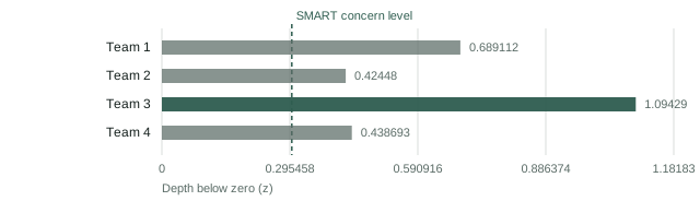
Mean weight-for-height z-score by measurement team, plotted as depth below zero. Clusters were assigned to teams independently of nutrition status, so a spread of this size between teams is a measurement fault rather than a real difference between populations. Speaker notes
Sex ratio near 1.0 — passes. Team means spread from -0.42 to -1.09. Fails. Clusters were assigned to teams independently of nutritional status, so a spread of 0.67 z-scores between teams is not a difference in the children; it is a difference in the measuring.Sex ratio and team bias — In Python
gam_by_team = (
    smart[smart["whz"].between(-5, 5)]
    .assign(gam=lambda d: (d["whz"] < -2) | (d["oedema"] == True))
    .groupby("team")["gam"].mean()
)
print((gam_by_team * 100).round(1))
Speaker notes
What it costs is direct:Sex ratio and team bias — In R
smart |>
  filter(between(whz, -5, 5)) |>
  summarise(gam = mean(whz < -2 | oedema), .by = team)
Speaker notes
Team 3's clusters give GAM of 22.3% against 9.2% to 16.2% for the others. Team 3 contributes a quarter of the sample and pulls the survey-wide estimate up by roughly two points.The verdict — In Python
plausibility = pd.DataFrame({ "check": ["Flagged records", "SD of WHZ", "Digit preference", "Age heaping", "Sex ratio", "Team bias"], "value": ["1.4%", "1.22", "69% (team 2)", "24% whole years", "1.05", "-0.42 to -1.09"], "acceptable": ["<2.5%", "0.8-1.2", "even across teams", "low", "~1.0", "close across teams"], "verdict": ["pass", "fail", "fail", "fail", "pass", "fail"], }) print(plausibility)The verdict — In R
tibble::tribble( ~check, ~value, ~verdict, "Flagged records", "1.4%", "pass", "SD of WHZ", "1.22", "fail", "Digit preference", "69% (team 2)", "fail", "Age heaping", "24%", "fail", "Sex ratio", "1.05", "pass", "Team bias", "-0.42 to -1.09", "fail" )The verdict
- Reject the survey. Defensible with four failures, and expensive — six weeks and a budget, gone.
- Accept with stated limitations. Report the prevalence with the plausibility table beside it and an explicit…
- Reanalyse excluding team 3. Defensible only if you say so prominently, and it costs a quarter of the sample and…
Speaker notes
Four failures. What follows is a judgement, not an arithmetic result, and the honest options are three: What you must not do is publish the prevalence without the plausibility report. The number is not wrong; it is unqualified, and the qualification changes what it supports.Write it up without accusing anyone
Do not write Write "Team 2's measurements are unreliable" "Team 2's height readings end in .0 or .5 in 69% of cases against 18-23% for other teams, consistent with reading the board to the nearest half centimetre" "Team 3 falsified measurements" "Team 3's mean weight-for-height is 0.4 to 0.7 z-scores below the other teams. Clusters were assigned independently of nutrition status, so this is most consistent with a measurement or calibration difference" "Ages are inaccurate" "24% of ages fall on an exact whole year against 9% expected, indicating age was estimated rather than documented for a substantial share of children" Speaker notes
The right-hand column names what was observed, its size and a mechanism. It is also what makes the corrective action obvious — recalibrate a scale, retrain on board reading, add an events calendar — where the left-hand column produces a defensive team and worse data next round.What comes next
- You know whether the survey can be believed and with what caveats.
Speaker notes
You know whether the survey can be believed and with what caveats. The next lesson turns it into the number it exists to produce — GAM and SAM prevalence, with an interval that accounts for the cluster design, read against the IPC phases.