Missingness that is not an accident

5.4% is not a finding

The register is missing age_months on 226 of 4,218 rows. Reported as “the dataset is 94.6% complete”, that number is worse than useless: it invites the reader to conclude the problem is small, and it is not small, because it is not spread out.

A completeness figure only means something once you know where the holes are. Scattered missingness costs precision. Clustered missingness costs the answer. This lesson is how to tell which one you have, and what to say about it.

Break it down by group before you do anything else

by_commune = (
    muac.assign(missing_age=muac["age_months"].isna())
    .groupby("commune")
    .agg(missing=("missing_age", "mean"), n=("missing_age", "size"))
    .sort_values("missing", ascending=False)
)
print((by_commune["missing"] * 100).round(1))

muac |>
  group_by(commune) |>
  summarise(missing = mean(is.na(age_months)), n = n()) |>
  arrange(desc(missing)) |>
  mutate(missing = round(100 * missing, 1))

Commune	Missing age	Rows
Gros-Morne	17.7%	361
Anse-Rouge	5.7%	229
Saint-Michel	5.1%	335
Dessalines	4.9%	450
Ennery	3.0%	263

Eleven communes sit between 3% and 6%. One sits at 17.7%. That is not a distribution with a long tail; it is eleven communes with a normal amount of missingness and one commune with a problem.

Then by time, inside the group that stands out

gros_morne = muac[muac["commune"] == "Gros-Morne"].copy()
gros_morne["week"] = gros_morne["screening_date"].dt.to_period("W").dt.start_time

print(
    gros_morne.groupby("week")["age_months"]
    .apply(lambda s: s.isna().mean())
    .sort_values(ascending=False)
    .head()
)

muac |>
  filter(commune == "Gros-Morne") |>
  mutate(week = lubridate::floor_date(screening_date, "week", week_start = 1)) |>
  group_by(week) |>
  summarise(missing = mean(is.na(age_months)), n = n()) |>
  arrange(desc(missing)) |>
  head()

The week beginning 10 June: 54 of 85 screenings, 63.5%. Every other week in that commune is under 10%.

That is no longer a data quality statistic. It is one team, one week, one tablet form with the age field misconfigured, and it has a name, a date and probably a person who remembers it. Missingness that resolves to an event is missingness you can ask about, and often fix at source.

Name the mechanism, in words the report can carry

The statistical literature has three categories. You do not need the notation, but you do need the distinction, because it decides what you are allowed to do.

• Missing completely at random. The holes are unrelated to anything, including the value that is missing. Dropping those rows costs precision and nothing else.
• Missing at random. The holes depend on something you observed — a commune, a week, an enumerator. Dropping them biases the result, but you can adjust for the thing they depend on, because you have it.
• Missing not at random. The holes depend on the missing value itself. The sickest children are the ones the queue never reached; the households that refused the water quality test are the ones with the dirtiest water. Nothing in the data can fix this, and the only honest response is to say so.

The age missingness here is missing at random: it depends on commune and week, both of which are recorded. The -99 MUAC codes may be worse than that — if measurement was skipped when a child was distressed, and distress correlates with illness, that is missing not at random, and no amount of code will tell you.

The category is not a statistical technicality. It is the difference between “we dropped 226 rows” and “we dropped 226 rows, 54 of them from one commune in one week, which moved that commune’s rate by 1.1 points”.

Put a number on what dropping them costs

This is the step almost nobody does, and it takes six lines. Compute the indicator twice: once on everything, once on complete cases only.

def gam_rate(df):
    assessed = df["muac_mm"].notna() | df["oedema"].notna()
    cases = assessed & ((df["muac_mm"] < 125) | (df["oedema"] == True))
    return pd.Series({
        "assessed": int(assessed.sum()),
        "cases": int(cases.sum()),
        "rate": round(cases.sum() / assessed.sum(), 3),
    })


all_rows = muac.groupby("commune").apply(gam_rate)
complete = muac[muac["age_months"].notna()].groupby("commune").apply(gam_rate)

comparison = all_rows.join(complete, rsuffix="_complete")
comparison["shift"] = comparison["rate_complete"] - comparison["rate"]
print(comparison.sort_values("shift"))

gam_rate <- function(df) {
  df |>
    mutate(
      assessed = !is.na(muac_mm) | !is.na(oedema),
      case     = assessed & (muac_mm < 125 | oedema)
    ) |>
    summarise(
      assessed = sum(assessed, na.rm = TRUE),
      cases    = sum(case, na.rm = TRUE),
      rate     = round(cases / assessed, 3),
      .by      = commune
    )
}

comparison <- gam_rate(muac) |>
  left_join(gam_rate(filter(muac, !is.na(age_months))),
            by = "commune", suffix = c("", "_complete")) |>
  mutate(shift = rate_complete - rate) |>
  arrange(shift)

Commune	All rows	Complete cases	Shift
Gros-Morne	14.5%	13.4%	-1.1 pt
Anse-Rouge	15.6%	16.5%	+0.9 pt
Dessalines	5.8%	5.4%	-0.4 pt
Saint-Michel	7.6%	7.6%	0.0 pt

Read the first two rows together. On all rows, Gros-Morne is second worst at 14.5% and 1.7 points clear of the commune below it. On complete cases it is 13.4%, and the commune below it is at 13.3%. The gap between second and third place goes from 1.7 points to 0.1 — which is to say, the ranking you would put in front of a nutrition cluster meeting depends on a form misconfiguration in one commune in June.

Notice also that nothing here crossed a threshold in a way that changed a decision. Say that too. A sensitivity check that finds no effect is a result, and it is the one that lets you stop worrying.

The three responses, and when each is honest

Drop them, and report the drop. Legitimate when the missingness is scattered and you have shown it is. The reporting is not optional: “n = 3,992 of 4,218; 226 rows excluded for missing age” belongs in the table footnote, not in your head.

Keep them, in a category of their own. Often the right answer for a categorical variable, because “not recorded” is a real finding about the programme. A completeness column beside the indicator column says more than either alone.

Impute — carefully, and rarely. For a variable used to disaggregate rather than to compute, filling missing age from the median age of the same commune and month is defensible if you flag every imputed row and report the indicator both ways. For a variable in the numerator, imputation is inventing the finding.

muac["age_imputed"] = muac["age_months"].isna()
muac["age_months_filled"] = muac.groupby("commune")["age_months"].transform(
    lambda s: s.fillna(s.median())
)

muac <- muac |>
  mutate(age_imputed = is.na(age_months)) |>
  group_by(commune) |>
  mutate(age_months_filled = ifelse(is.na(age_months),
                                    median(age_months, na.rm = TRUE),
                                    age_months)) |>
  ungroup()

The flag column is the point. An imputed value that is indistinguishable from a measured one has stopped being an estimate and started being a claim.

Missing rows, not just missing values

The hardest missingness is the kind with no blank cell, because the row is not there at all.

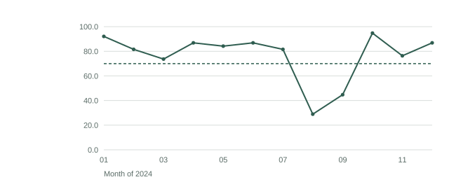
In the routine vaccination extract, a facility that did not report is not absent — it is present with doses_administered of zero and report_submitted of false. Six hundred and forty-two rows are in that state. Compute coverage without separating them and every non-reporting facility becomes a facility that vaccinated nobody.

vax["reported"] = vax["report_submitted"] == True

reporting_rate = vax.groupby("period")["reported"].mean()
coverage = (
    vax[vax["reported"]]
    .groupby("period")
    .apply(lambda g: g["doses_administered"].sum() / g["target_population"].sum())
)
print(pd.DataFrame({"reporting_rate": reporting_rate, "coverage": coverage}))

vax |>
  summarise(
    reporting_rate = mean(report_submitted),
    coverage = sum(doses_administered[report_submitted]) /
               sum(target_population[report_submitted]),
    .by = period
  )

Two numbers, always published together. Coverage computed on facilities that reported, and the reporting rate that says how much of the district that covers. A single coverage figure that quietly includes silent facilities in its denominator is the most common defect in routine health data, and it always points the same way — down.

What comes next

Missingness is a hole where something should be. The next unit is the opposite problem: something that is there twice. Lesson 3 asks whether the column you have been treating as a key actually is one — and shows what a join does when it is not.