Twelve communes, one ranking, eleven overlapping intervals

The ranking the chart invites

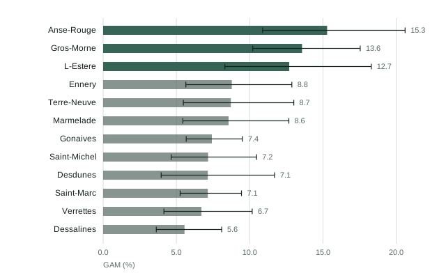
Twelve communes, sorted, from 15.3% down to 5.6%. Without the whiskers this is a league table: someone is worst, someone is best, and a targeting decision follows.

import pandas as pd

communes = pd.DataFrame({
    "commune": ["Anse-Rouge", "Gros-Morne", "L-Estere", "Ennery", "Terre-Neuve",
                "Marmelade", "Gonaives", "Saint-Michel", "Desdunes",
                "Saint-Marc", "Verrettes", "Dessalines"],
    "gam":  [.153, .136, .127, .088, .087, .086, .074, .072, .071, .071, .067, .056],
    "low":  [.109, .102, .083, .056, .055, .054, .057, .046, .040, .053, .041, .036],
    "high": [.206, .175, .183, .129, .130, .127, .095, .105, .117, .094, .102, .081],
})

overlaps = sum(communes["high"][i] > communes["low"][i - 1]
               for i in range(1, len(communes)))
print(f"adjacent pairs whose intervals overlap: {overlaps} of {len(communes) - 1}")

# Eleven of eleven. The ranking is a ranking of point estimates only.

Every adjacent pair overlaps. The chart can support “these three are higher than the district median” and cannot support “Gros-Morne is worse than L’Estère”.

The interval is what converts a ranking into a finding. Without it, the reader supplies an ordering the data does not contain, and the more carefully the bars are sorted the more convincing the invented ordering looks.

Drawing the interval

import matplotlib.pyplot as plt

fig, ax = plt.subplots(figsize=(7, 4))
ax.barh(communes["commune"], communes["gam"])
ax.errorbar(communes["gam"], communes["commune"],
            xerr=[communes["gam"] - communes["low"],
                  communes["high"] - communes["gam"]],
            fmt="none", capsize=3)
ax.invert_yaxis()

ggplot(communes, aes(x = gam, y = reorder(commune, gam))) +
  geom_col() +
  geom_errorbarh(aes(xmin = low, xmax = high), height = 0.3)

Four decisions, each of which changes what the reader concludes.

Say what the interval is. “95% confidence interval” in the caption, every time. A bare whisker is read as a standard error by some readers, a range by others, and a minimum and maximum by most.

Use the right interval. These are Clopper–Pearson exact binomial intervals, because several communes have small denominators and the Wald interval the statistics course rejected produces bounds below zero on exactly those cells.

Do not clip a bound to make it fit. An interval that reaches 20.6% sets the axis; truncating the axis to 15% and letting the whisker run off the edge is a chart that has hidden its own uncertainty.

Whiskers on top of bars, not instead of them. For a proportion the bar carries the magnitude and the whisker carries the doubt. A dot-and-whisker plot is equally defensible and reads better above about fifteen categories.

When intervals are not the right encoding

Three cases, and reaching for a whisker in any of them is worse than leaving it off.

A census, not a sample. A count of every water point in a district has no sampling error. It has other errors — a point missed, a status recorded wrongly — and a confidence interval does not describe them. Say the denominator is complete instead.

A total, not a rate. “1,850 cases registered” is a count of what happened. It carries no interval, and the protection course spent a lesson on why.

A time series a reader has to see the shape of. Twelve monthly points with whiskers becomes a hedge; a shaded band behind the line is the same information and leaves the shape legible.

ax.fill_between(months, lower, upper, alpha=0.2)
ax.plot(months, values)

geom_ribbon(aes(ymin = lower, ymax = upper), alpha = 0.2) + geom_line()

The reference line does more work than the intervals

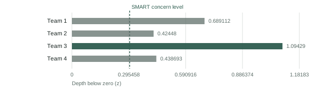
A number is compared against something whether or not you draw it, and drawing it decides what.

Sphere thresholds, SMART concern levels, IPC phase boundaries, national targets, a previous round. Each is a reference someone in the room is holding, and the chart that draws it is the chart everyone is looking at the same way.

Label the line with what it is, not with its value. “70% floor” beats “0.70”, which the reader can already see on the axis.

One reference line. Two is a comparison the reader has to perform; three is decoration.

Reading order, and the three that clear

The figure marks three communes rather than describing them, which is a decision worth copying.

median = communes["gam"].median()
clears = communes[communes["low"] > median]
print(f"median {median:.1%}; clearing it: {list(clears['commune'])}")

communes |> filter(low > median(gam)) |> pull(commune)

Anse-Rouge, Gros-Morne and L’Estère are the only three whose lower bound exceeds the district median of 8.0%. That is a defensible statement and it is the one the highlight makes. Everything below them is a group, not a sequence.

Emphasis is an argument, so make it the argument the caption makes. Highlighting the top three by value would have marked the same three here by luck; highlighting by whether the interval clears the median marks them for a reason, and the two would diverge on a different dataset.

Report it whole

Global acute malnutrition by commune, Artibonite, 2024

  Prevalence by commune with 95% Clopper-Pearson intervals, sorted by point
  estimate. n ranges from 189 to 768 screenings per commune.

  Three communes -- Anse-Rouge, Gros-Morne and L'Estere -- have lower bounds
  above the district median of 8.0% and are highlighted.

  All eleven adjacent pairs have overlapping intervals. The chart supports
  "these three are above the district median" and does not support a ranking
  of one commune against its neighbour.

  Intervals are exact binomial. Communes with fewer than 300 screenings have
  intervals roughly twice as wide as Gonaives and Saint-Marc, which is a
  property of where the screening teams went rather than of their nutrition
  situation.

The third paragraph is what stops the chart being used as a league table, and it is the sentence a reader will not supply for themselves.

What comes next

Both figures in this lesson use one colour for the ordinary bars and one for the emphasised ones. The next lesson is about the three colours they deliberately do not use, and why spending them on districts costs something that cannot be bought back.