Lesson 1 of 8
Unit · The mark and the comparison
The comparison decides the mark
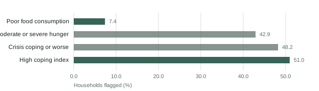
Four food security instruments on the same 1,955 households give 7.4%, 42.9%, 48.2% and 51.0%. Written as a sentence a reader nods; drawn as four bars nobody reads past it. The chart type was decided by the comparison, not by preference.
Start from the sentence, not the library
Before any plotting code, write the sentence the chart is making. The mark follows from it almost mechanically.
| The sentence compares | Mark | Why |
|---|---|---|
| Categories against each other | Sorted horizontal bar | Length is the most accurately read encoding, and labels fit |
| One quantity over time | Line | Slope is the comparison; a bar chart of months hides it |
| A part against its whole | A single bar, or the number | A pie is two numbers and a legend |
| Two continuous variables | Scatter | Position on both axes |
| The same comparison across places | Small multiples | One shape repeated, read once |
| Where something stops | Ordered stages | The drop between bars is the finding |
Nothing on this platform has yet needed a mark outside that list, which is a fact about programme reporting rather than about the list: the comparisons a programme makes are overwhelmingly categorical, temporal, or a proportion with an interval on it.
The four-instrument chart
import pandas as pd
import matplotlib.pyplot as plt

prevalence = pd.Series({
    "Poor food consumption": 0.074,
    "Moderate or severe hunger": 0.429,
    "Crisis coping or worse": 0.482,
    "High coping index": 0.510,
})

fig, ax = plt.subplots(figsize=(7, 2.6))
ax.barh(prevalence.index, prevalence.values)
ax.invert_yaxis()                       # first row at the top
ax.set_xlabel("Households flagged (%)")library(ggplot2)
ggplot(prevalence, aes(x = share, y = reorder(instrument, share))) +
geom_col() +
labs(x = "Households flagged (%)", y = NULL)Horizontal, because the labels are words. “Moderate or severe hunger” rotated 45 degrees under a vertical bar is a chart that has decided its own labels are less important than its bars.
Sorted, unless the order means something. Alphabetical order is an ordering nobody asked about. Here the natural order is by value, and the sorted version makes the seven-fold gap the first thing seen.
One exception worth knowing. When the categories have their own order — IPC phases, MUAC bands, months, education grades — sorting by value destroys information the reader already has. Sort by value, or by the category’s own order, and never by the alphabet.
The chart that is a table
coverage = pd.Series({"Measles first dose": 0.87, "Measles second dose": 0.61})# Two numbers. A chart of two numbers is a chart of nothing.Two or three numbers belong in a sentence. “Coverage falls from 87% to 61% between the first and second dose” is faster to read than any chart of it, occupies one line, and cannot be misread from the back of a room.
A chart earns its space at about five categories and stops being read at about twenty-five. Below five, write the sentence. Above twenty-five, you are drawing a table and should draw a table — or aggregate, which is a finding rather than a formatting choice.
Where something stops
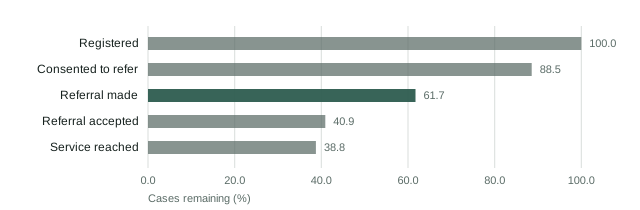
A pathway is a sequence of stages, each a subset of the last, and the useful question is where the largest loss happens.
stages = pd.Series({
    "Registered": 1.000, "Consented to refer": 0.885, "Referral made": 0.617,
    "Referral accepted": 0.409, "Service reached": 0.388,
})
losses = -stages.diff().dropna()
print(losses.round(3))
print(f"largest drop: {losses.idxmax()} ({losses.max():.1%})")
# The drop is the finding; the bars are how you show it.The largest single drop is 26.8 points, between consent and a referral being made. Not at the service, not at acceptance — at the point where a caseworker decides whether to refer at all.
Bars in stage order, never sorted. The sequence is the meaning. And the figure marks the biggest drop, because a reader scanning five descending bars will otherwise take the last one as the story.
Three marks to avoid, and what to use instead
The pie chart. Angles are read less accurately than lengths, and a pie with more than three slices needs a legend to be read at all. Use a sorted bar. The one defensible pie is a single proportion against its complement, and a sentence beats that too.
The dual-axis chart. Two series on two scales, and the crossing point is decided by where you put the axes. Use two small charts stacked, sharing an x-axis, so a reader can see both without being told a relationship the scaling invented.
The 3-D anything. Depth adds no data and distorts every length it touches.
# The one line of matplotlib configuration this course insists on.
plt.rcParams.update({"axes.spines.top": False, "axes.spines.right": False})theme_set(theme_minimal(base_size = 11))The stacked bar, which is sometimes right
Stacking is the one contested case, so it is worth being precise.
Stacked bars are readable for the bottom segment and unreadable above it. Every segment except the first starts at a different baseline, so comparing the third segment across bars is comparing lengths that begin nowhere in particular.
Use stacking when the total matters and the composition is secondary — a caseload split by category, where the reader’s first question is how big the caseload is. Use grouped bars or small multiples when a specific component is the question.
Never stack percentages that do not sum to 100. The four instruments above overlap: a household can be flagged by three of them. Stacking those four would draw a bar of 149.5% and imply a whole nobody has.
Report it whole
Food security instruments, 1,955 households, 2024

  Four instruments were applied to the same households and are shown as a
  sorted horizontal bar chart. The bars are prevalences, not components of a
  total: households can be flagged by more than one instrument, so the bars
  do not sum and are not stacked.

  Poor food consumption            7.4%
  Moderate or severe hunger       42.9%
  Crisis coping or worse          48.2%
  High coping index               51.0%

  The chart's claim is the spread, not any single bar. 76.3% of households
  are flagged by at least one instrument and 3.4% by all four.
The second paragraph is the one that stops the chart being misread, and it is two sentences. A reader who assumes those four bars are parts of something will build a caseload out of them.
What comes next
Every bar in this lesson is a proportion estimated from a sample, and not one of them carries an interval. The next lesson puts them on, and finds that the ordering of a twelve-commune chart survives it in only three cases.