A gap of half a point, filling half the chart

The same two numbers, four charts

The statistics course established that the attendance gap between boys and girls is 0.56 percentage points — significant at p = 0.023 on 68,267 marks, and equal to about a third of one school day per child per term.

import matplotlib.pyplot as plt

rates = {"Boys": 0.8877, "Girls": 0.8821}
gap = (rates["Boys"] - rates["Girls"]) * 100

for lo, hi in [(0, 100), (80, 95), (87.5, 89.5), (88, 89)]:
    share = gap / (hi - lo) * 100
    print(f"axis {lo}-{hi}: the gap fills {share:.1f}% of the chart height")

# Same data, four y-limits, four different stories.

Axis	The gap occupies	Magnification
0 to 100	0.6% of the chart	×1
80 to 95	3.7%	×7
87.5 to 89.5	27.8%	×50
88 to 89	55.7%	×100

Every one of those charts is accurate. The bars are in the right places, the axis is labelled, the numbers are correct. The last one shows a difference that no programme would act on filling more than half the plotting area.

Truncating a bar chart’s axis is the single most effective way to mislead with correct data, and it is done far more often by accident than by design.

The rule, and the exception

A bar chart’s value axis starts at zero. Always. A bar encodes its quantity as a length, and a length measured from a moving origin is not a quantity. This is not a convention with exceptions; it is what makes a bar readable.

A line chart’s axis does not have to. A line encodes change as slope, and the reader is comparing points to each other rather than to the origin. A temperature series starting at zero degrees is a flat line and a wasted chart.

fig, (a, b) = plt.subplots(1, 2, figsize=(9, 3))
a.bar(rates.keys(), rates.values())         # must include zero
a.set_ylim(0, 1)
b.plot(months, completeness)                # need not include zero
b.set_ylim(0.25, 1.0)

# geom_col() + expand_limits(y = 0). geom_line() + coord_cartesian(ylim = ...).

And when you truncate a line’s axis, say so on the axis. A break mark, or an axis label that starts visibly above zero, or a note. The reader who assumes zero and is wrong has read the chart backwards.

When the truncation is the honest choice

The completeness figure is the case, and it is worth being precise about why.

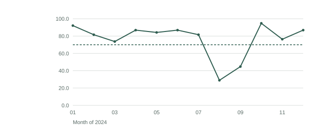
values = [.921, .816, .737, .868, .842, .868, .816, .289, .447, .947, .763, .868]
print(f"range {min(values):.1%} to {max(values):.1%}")

range(values)

Completeness runs from 28.9% to 94.7% — a range of 65.8 points across a 100-point axis. The data uses two-thirds of the available height, so a zero-based axis wastes almost nothing and the shape is fully legible.

The rule to apply is: does the truncation change how large the variation looks? Here it barely would, so there is no argument for it. Where truncation would magnify a 0.5-point difference into half a chart, the answer is not to truncate more carefully — it is that a bar chart was the wrong mark and the number belongs in a sentence.

Five more axis decisions that change the reading

Reversed axes. A rate where lower is better — mortality, defaulting, stunting — drawn with the worst value at the top reads as a success. Say which direction is good in the axis label: “Defaulter rate (%), lower is better”.

Log scales. Legitimate for an outbreak curve spanning three orders of magnitude, and misread by almost every non-technical audience as a linear one. If you use one, label it and annotate a doubling.

Percentage axes above 100. Gross enrolment reaches 109.2% in the education course’s data, and an axis capped at 100 clips the bar and hides the finding.

Time axes with uneven spacing. Twelve monthly points drawn at even spacing when two months are missing draws a straight line through a gap. Plot the dates, not the sequence.

Aspect ratio. The same line at twice the height looks twice as steep. There is no neutral choice, so pick one and use it for every chart in the report, which at least makes them comparable to each other.

fig.set_size_inches(6.5, 4)      # every figure in the report, the same shape

# ggsave(width = 6.5, height = 4) as a project default.

The missing-data trap, which is an axis problem

The completeness figure exists because of this and it is worth stating directly.

A month with no reports drawn as zero is a claim that nothing happened. A month with no reports left out of the series entirely is a claim that time did not pass. Neither is true, and the honest chart shows the gap.

series = series.reindex(all_months)          # missing months become NaN
ax.plot(series.index, series.values)          # matplotlib breaks the line at NaN

# Do not tidyr::replace_na(0). A gap is data about the reporting system.

August’s 28.9% is a reporting failure, not an epidemiological one. The epidemiology course spent a lesson on it, and the chart’s job is to make it look like what it is — a hole in the denominator — rather than like a fall in cases.

Report it whole

Figure axis conventions

  Bar charts use zero-based value axes without exception. Where a difference
  is too small to be visible on a zero-based axis, it is reported as a
  sentence rather than as a chart.

  Line charts may use a truncated axis where the data range justifies it; the
  axis is labelled so the truncation is visible.

  Indicators where lower is better carry "lower is better" in the axis label.

  Months with no data are drawn as gaps, never as zero. Completeness is
  reported alongside any indicator whose denominator varies by month.

  All figures in this report are drawn at 6.5 by 4 inches, so vertical
  changes are comparable between charts.

The first paragraph is the one worth adopting verbatim. “Report it as a sentence rather than as a chart” is the decision that would have prevented the 88-to-89 chart, and it is a decision about honesty rather than about design.

What comes next

Every rule in this course is a rule someone has to remember on the day they make the chart. The last lesson removes the remembering, by generating the figure from the dataset — which is how every chart on this platform is built and why none of them can drift from the sentence beside it.