Lesson 5 of 8
Unit · Making it trustworthy
Finding what is wrong with the data
Profile a fresh export systematically — missingness by site and week, implausible measurements, duplicates with no clean key, and codes that contradict each other.
Profile before you analyse
You have a tidy table with the right types. You do not yet know what is in it.
The instinct is to compute the indicator and look at the number. Resist it: the number will be plausible whatever is wrong, and once you have seen it you will find reasons to believe it. Profile first, decide second, compute third.
This lesson is the profiling. Five checks, in order of how much damage they do when missed.
Check 1: completeness, by group and not overall
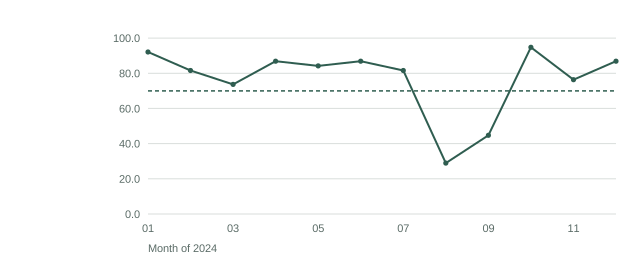
A facility that did not report appears in the extract as rows of zeroes, so a completeness chart and a coverage chart tell you different things — and reading the second without the first is how a silent facility becomes a failing one. Note also that two months move together: whatever happened there is a district event, and a quality flag raised against individual facilities in that window would be pointing at the wrong thing.
A single completeness figure is nearly useless. What matters is whether the missingness clusters, because clustered missingness biases and scattered missingness mostly just costs precision.
overall = muac.isna().mean().sort_values(ascending=False)
print(overall)

by_commune = (
    muac.assign(missing_age=muac["age_months"].isna())
    .groupby("commune")["missing_age"]
    .agg(["mean", "size"])
    .sort_values("mean", ascending=False)
)
print(by_commune)
muac |>
summarise(across(everything(), ~ mean(is.na(.x)))) |>
tidyr::pivot_longer(everything(), names_to = "column", values_to = "missing") |>
arrange(desc(missing))
muac |>
group_by(commune) |>
summarise(
missing_age = mean(is.na(age_months)),
n = n()
) |>
arrange(desc(missing_age))Run it on this register and the overall missingness of age_months is about 5%,
which sounds tolerable. Break it down and Gros-Morne is far worse than the
others. Break it down by week as well and it collapses onto a single campaign
week, 10 to 14 June:
gros_morne = muac[muac["commune"] == "Gros-Morne"].copy()
gros_morne["week"] = gros_morne["screening_date"].dt.to_period("W")

print(
    gros_morne.groupby("week")["age_months"]
    .apply(lambda s: s.isna().mean())
    .sort_values(ascending=False)
    .head()
)
muac |>
filter(commune == "Gros-Morne") |>
mutate(week = lubridate::floor_date(screening_date, "week")) |>
group_by(week) |>
summarise(missing_age = mean(is.na(age_months)), n = n()) |>
arrange(desc(missing_age))That is not a data quality nuisance. It is one team, one week, one tablet form that had the age field misconfigured — and it means that dropping incomplete rows removes Gros-Morne far more than any other commune. If you then rank communes by malnutrition rate, you have ranked them partly on which team’s form was broken.
Missingness that clusters in one site or one week is the difference between losing precision and losing the answer. Always break it down before you decide what to do with it.
Check 2: implausible values
Every sector has physical limits. Use them.
For MUAC in children 6 to 59 months, values below about 80 mm or above about 220 mm are not measurements — they are recording errors. The register carries seven records where the measurement was left in centimetres and never converted, which appear as values below 40.
implausible = muac[(muac["muac_mm"] < 80) | (muac["muac_mm"] > 220)]
print(implausible[["child_id", "commune", "age_months", "muac_mm"]])

print(muac["muac_mm"].describe())
muac |>
filter(muac_mm < 80 | muac_mm > 220) |>
select(child_id, commune, age_months, muac_mm)
summary(muac$muac_mm)A value of 13.3 where you expected 133 is a unit error, and it is recoverable — you know what it was meant to be. A value of 450 is not recoverable and has to be treated as missing. Distinguishing the two is a judgement call, which is why it belongs in the cleaning log rather than in a one-line filter.
Check the age range too. A MUAC screening programme targets 6 to 59 months, so a row recording 72 months is either out of scope or a data entry error, and which one it is changes your denominator.
print(muac["age_months"].describe())
print(muac[(muac["age_months"] < 6) | (muac["age_months"] > 59)].shape[0])summary(muac$age_months)
sum(muac$age_months < 6 | muac$age_months > 59, na.rm = TRUE)Check 3: duplicates, including the ones without a clean key
Exact duplicates are easy:
exact = muac[muac.duplicated(keep=False)]
print(f"{len(exact)} rows in exact-duplicate groups")

repeated_ids = muac[muac.duplicated(subset=["child_id"], keep=False)]
print(f"{len(repeated_ids)} rows sharing a child_id")sum(duplicated(muac))
muac |>
group_by(child_id) |>
filter(n() > 1) |>
arrange(child_id)This register has twelve exact duplicates, from forms submitted twice on a poor connection. Those are unambiguous — the same submission arrived twice, and one copy should go.
The harder case is a child re-registered under a new identifier, which shares no key at all. Six of those are in this file, findable only by matching on the attributes that should not coincide by chance:
suspects = (
    muac.groupby(["commune", "screening_date", "age_months", "sex", "muac_mm"])
    .filter(lambda g: len(g) > 1)
    .sort_values(["commune", "screening_date", "muac_mm"])
)

print(suspects[["child_id", "commune", "screening_date", "age_months", "sex", "muac_mm"]])
muac |>
group_by(commune, screening_date, age_months, sex, muac_mm) |>
filter(n() > 1) |>
arrange(commune, screening_date, muac_mm) |>
select(child_id, commune, screening_date, age_months, sex, muac_mm)Be careful here: two different children of the same age and sex, screened in the
same commune on the same day, with the same MUAC to the millimetre, is possible.
In a large campaign it is even likely. This check produces suspects, not
duplicates, and the resolution is a human looking at the register — not a
drop_duplicates() call.
Check 4: internal contradictions
Columns that should agree, and do not. This register has two such faults.
Seventy-three records carry a referral outcome but no MUAC value — the decision column and the measurement column were filled by different people:
contradiction_a = muac[
    muac["outcome"].isin(["referred-tsfp", "referred-otp", "referred-sc"])
    & muac["muac_mm"].isna()
]
print(len(contradiction_a))
muac |>
filter(outcome %in% c("referred-tsfp", "referred-otp", "referred-sc"),
is.na(muac_mm)) |>
nrow()And nine records carry an outcome that contradicts their own measurement — a child measured at 140 mm marked as referred to outpatient therapeutic care, or a child at 110 mm marked no-action. This is what a mis-tapped tablet screen produces.
def expected_outcome(row):
    if pd.isna(row["muac_mm"]):
        return None
    if row["oedema"] is True or row["muac_mm"] < 115:
        return "referred-otp"
    if row["muac_mm"] < 125:
        return "referred-tsfp"
    return "no-action"

check = muac.assign(expected=muac.apply(expected_outcome, axis=1))
mismatched = check[
    check["expected"].notna()
    & (check["expected"] == "no-action")
    & (check["outcome"] != "no-action")
]
print(len(mismatched))
muac |>
mutate(
expected = case_when(
is.na(muac_mm) ~ NA_character_,
oedema | muac_mm < 115 ~ "referred-otp",
muac_mm < 125 ~ "referred-tsfp",
TRUE ~ "no-action"
)
) |>
filter(!is.na(expected), expected == "no-action", outcome != "no-action") |>
nrow()Note that this check encodes a clinical rule. It is only as good as the rule, and referral to a stabilisation centre depends on complications the register does not record — so treat a mismatch as a flag for review, not as proof the outcome is wrong.
Check 5: inconsistent coding of the same thing
The oedema column is recorded as true/false for most of the file, but
Ennery and Desdunes used Y/N in the first quarter, and some rows are blank.
raw = pd.read_csv(PATH, dtype={"oedema": "string"})
print(raw.groupby("commune")["oedema"].value_counts(dropna=False))read_csv(PATH, col_types = cols(.default = col_character())) |>
count(commune, oedema)Always look at the raw string values of a categorical column before converting. Converting first and counting the missing afterwards tells you how many rows had an unexpected value; looking at the raw values tells you what they were, which is what you need to decide whether they are recoverable.
A profile function worth keeping
Wrap the whole thing so it runs on every new export without being retyped.
def profile(df, group=None):
    report = {
        "rows": len(df),
        "columns": df.shape[1],
        "duplicate_rows": int(df.duplicated().sum()),
        "missing": df.isna().mean().round(4).to_dict(),
    }
    if group:
        report["missing_by_group"] = (
            df.isna().groupby(df[group]).mean().round(4).to_dict("index")
        )
    return report


import json
print(json.dumps(profile(muac, group="commune"), indent=2, default=str))
profile <- function(df, group = NULL) {
out <- list(
rows = nrow(df),
columns = ncol(df),
duplicate_rows = sum(duplicated(df)),
missing = sapply(df, function(x) round(mean(is.na(x)), 4))
)
if (!is.null(group)) {
out$missing_by_group <- df |>
group_by(.data[[group]]) |>
summarise(across(everything(), ~ round(mean(is.na(.x)), 4)))
}
out
}
str(profile(muac, group = "commune"))Run this on every export, save the output next to the data, and you have a record of what the file looked like on arrival. That record is what lets you answer “was this always like that?” six months later.
What comes next
You now know what is wrong. The next lesson is about deciding what to do about each fault — and, more importantly, about writing those decisions down in a form that survives the person who made them.