Lesson 7 of 8
Unit · Producing an answer
From tidy data to an indicator table
Turn a clean dataset into the disaggregated indicator table a logframe asks for, with numerator, denominator and confidence interval stated explicitly.
An indicator is a numerator over a denominator, disaggregated
That sentence is the whole lesson. Most reporting disputes are really disagreements about the denominator, and most of the rest are disagreements about which rows belong in the numerator.
So before any code: write the definition down.
The indicator reference sheet
For every indicator you report, fill this in. It takes five minutes and it ends the argument before it starts.
| Field | For our example |
|---|---|
| Indicator | Global acute malnutrition (GAM) prevalence by MUAC |
| Numerator | Children 6-59 months screened with MUAC below 125 mm, or with bilateral pitting oedema |
| Denominator | Children 6-59 months with a valid MUAC measurement or a recorded oedema assessment |
| Disaggregation | Commune, sex, age band (6-23, 24-59 months) |
| Frequency | Quarterly, and annually for the donor report |
| Source | Community mass screening register, CommCare |
| Decision it informs | Which communes receive an additional CMAM site next quarter |
| Reference value | GAM at or above 15% is the emergency threshold |
Note what the denominator is not. It is not all children in the commune — that would be coverage-adjusted prevalence and requires a population figure this register does not have. It is not all rows in the file — that would include rows with no measurement at all. Being explicit about this is what stops the number being quietly redefined between one report and the next.
If you cannot write the denominator in one sentence, you do not yet have an indicator. You have a column you are about to average.
Build the numerator as a column
Do not filter. Create a flag, keep every row, and let the aggregation do the work — that way the denominator is visible in the same table as the numerator.
import numpy as np

SAM_MM = 115
GAM_MM = 125

muac["has_assessment"] = muac["muac_mm"].notna() | muac["oedema"].notna()

muac["sam"] = np.where(
    ~muac["has_assessment"],
    np.nan,
    ((muac["muac_mm"] < SAM_MM) | (muac["oedema"] == True)).astype(float),
)

muac["gam"] = np.where(
    ~muac["has_assessment"],
    np.nan,
    ((muac["muac_mm"] < GAM_MM) | (muac["oedema"] == True)).astype(float),
)
SAM_MM <- 115
GAM_MM <- 125
muac <- muac |>
mutate(
has_assessment = !is.na(muac_mm) | !is.na(oedema),
sam = if_else(has_assessment, (muac_mm < SAM_MM) | oedema %in% TRUE, NA),
gam = if_else(has_assessment, (muac_mm < GAM_MM) | oedema %in% TRUE, NA)
)Two details that are easy to get wrong and expensive to miss:
- Oedema is SAM regardless of measurement. A child at 130 mm with bilateral
pitting oedema is severely acutely malnourished. Filtering on
muac_mmalone understates the caseload, and it understates it precisely among the most severe cases. oedema == Truerather than a truthiness test. Missing oedema is not false. In R,oedema %in% TRUEtreatsNAas not-oedema for the flag while keeping it distinguishable elsewhere; in Python the explicit comparison does the same.
The indicator table
def indicator_table(df, by):
    grouped = df.groupby(by, dropna=False)
    table = grouped.agg(
        screened=("child_id", "size"),
        denominator=("has_assessment", "sum"),
        sam_cases=("sam", "sum"),
        gam_cases=("gam", "sum"),
    )
    table["gam_rate"] = table["gam_cases"] / table["denominator"]
    table["sam_rate"] = table["sam_cases"] / table["denominator"]
    return table.reset_index()


by_commune = indicator_table(muac, "commune").sort_values(
    "gam_rate", ascending=False
)
print(by_commune.round(4))
indicator_table <- function(df, by) {
df |>
group_by(across(all_of(by))) |>
summarise(
screened = n(),
denominator = sum(has_assessment),
sam_cases = sum(sam, na.rm = TRUE),
gam_cases = sum(gam, na.rm = TRUE),
.groups = "drop"
) |>
mutate(
gam_rate = gam_cases / denominator,
sam_rate = sam_cases / denominator
)
}
by_commune <- indicator_table(muac, "commune") |> arrange(desc(gam_rate))
by_communeThe table carries screened and denominator as separate columns on purpose.
They differ by the rows with no assessment at all, and a reader who can see both
can tell how much of the register the rate is based on. A table that reports
only the rate hides that entirely.
Run it and the overall GAM rate lands near 8.6% with SAM near 2.2%, ranging from roughly 5% to 15% across communes. One commune crosses the 15% emergency threshold; the best does not come close. Those figures are stated in the dataset’s quality notes precisely so you can check your working against them — if your GAM comes out at 30%, you have a bug, not a famine.
Disaggregation
The logframe asked for commune, sex and age band. Age band needs constructing, and the boundaries are a choice you should state.
muac["age_band"] = pd.cut(
    muac["age_months"],
    bins=[6, 24, 60],
    labels=["6-23 months", "24-59 months"],
    right=False,
)

by_sex = indicator_table(muac, ["commune", "sex"])
by_age = indicator_table(muac, "age_band")

print(by_age.round(4))
muac <- muac |>
mutate(
age_band = cut(
age_months,
breaks = c(6, 24, 60),
labels = c("6-23 months", "24-59 months"),
right = FALSE
)
)
by_sex <- indicator_table(muac, c("commune", "sex"))
by_age <- indicator_table(muac, "age_band")
by_ageright = FALSE makes the bands left-closed: 6 to 23 completed months, then 24
to 59. Getting this backwards puts 24-month-olds in the younger band, which
shifts every rate slightly and is invisible in the output. State the convention
in the reference sheet.
Remember the missing-age problem from lesson 5. The age disaggregation necessarily excludes rows with no age, and Gros-Morne is over-represented among those. Report the age table with that caveat attached, or report it excluding Gros-Morne and say so.
Say how uncertain you are
A rate from 340 children is not the same claim as a rate from 12. Attach an interval.
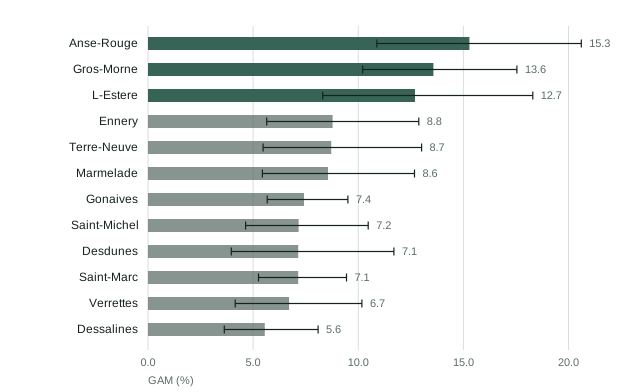
Read the whiskers, not the order. Nine of these twelve communes have overlapping intervals, which means the screening does not support a claim that any one of them is worse than another. A table sorted by rate invites exactly that claim, and the figure is the fastest way to stop it: the three bars whose interval clears the median are a finding, and the gap between the fourth and fifth is not.
from scipy.stats import beta

def wilson_interval(successes, n, confidence=0.95):
    if n == 0:
        return (np.nan, np.nan)
    lower = beta.ppf((1 - confidence) / 2, successes, n - successes + 1) if successes > 0 else 0.0
    upper = beta.ppf(1 - (1 - confidence) / 2, successes + 1, n - successes) if successes < n else 1.0
    return (lower, upper)


bounds = by_commune.apply(
    lambda r: wilson_interval(r["gam_cases"], r["denominator"]), axis=1
)
by_commune["gam_low"] = [b[0] for b in bounds]
by_commune["gam_high"] = [b[1] for b in bounds]

print(by_commune[["commune", "denominator", "gam_rate", "gam_low", "gam_high"]].round(4))
ci <- function(cases, n) {
if (n == 0) return(c(NA_real_, NA_real_))
test <- binom.test(cases, n)
test$conf.int
}
by_commune <- by_commune |>
rowwise() |>
mutate(
gam_low = ci(gam_cases, denominator)[1],
gam_high = ci(gam_cases, denominator)[2]
) |>
ungroup()
by_commune |> select(commune, denominator, gam_rate, gam_low, gam_high)Now look at the ranking again. Several communes have overlapping intervals, which means the ordering between them is not supported by the data. If the decision this table informs is “which commune gets the additional CMAM site”, that matters enormously — and a table without intervals would have let you rank them with false confidence.
This is also a census of those screened rather than a probability sample, so the interval describes sampling variation only. It says nothing about whether the children who came to be screened resemble the children who did not, which is usually the larger source of error and belongs in the limitations section.
Format it for the report
report = by_commune.assign(
    gam=lambda d: (d["gam_rate"] * 100).round(1).astype(str) + "%",
    ci=lambda d: "("
    + (d["gam_low"] * 100).round(1).astype(str)
    + " - "
    + (d["gam_high"] * 100).round(1).astype(str)
    + ")",
)[["commune", "screened", "denominator", "gam_cases", "gam", "ci"]]

report.columns = [
    "Commune", "Screened", "Assessed", "GAM cases", "GAM rate", "95% CI",
]
report.to_csv("output/tables/gam-by-commune.csv", index=False)
print(report.to_string(index=False))
report <- by_commune |>
transmute(
Commune = commune,
Screened = screened,
Assessed = denominator,
`GAM cases` = gam_cases,
`GAM rate` = sprintf("%.1f%%", gam_rate * 100),
`95% CI` = sprintf("(%.1f - %.1f)", gam_low * 100, gam_high * 100)
)
readr::write_csv(report, "output/tables/gam-by-commune.csv")
reportEvery column in that table is defensible: you can say where each number came from, what it counted, what it did not, and how uncertain it is.
What comes next
The last lesson makes this run again — on next quarter’s export, on someone else’s laptop, without editing anything.