Grouping to a numerator and a denominator

An indicator is two numbers

Almost every figure this sector reports is a numerator over a denominator, and almost every argument about a figure is an argument about the denominator. The practical consequence for your code: compute both in the same operation.

Two separate calculations drift. One gets a filter the other does not, someone edits one line, and the ratio becomes a number nobody can reconstruct.

import pandas as pd

muac = read_register(RAW / "muac-screening-artibonite-2024.v1.csv")

measured = muac["muac_mm"].notna()
gam = measured & (muac["muac_mm"] < 125)

by_commune = (
    muac.assign(measured=measured, gam=gam)
    .groupby("commune")
    .agg(
        screened=("child_id", "size"),
        measured=("measured", "sum"),
        gam_cases=("gam", "sum"),
    )
)
by_commune["gam_rate"] = (by_commune["gam_cases"] / by_commune["measured"]).round(3)

             screened  measured  gam_cases  gam_rate
commune
Gros-Morne        361       351         48     0.137
Anse-Rouge        229       223         30     0.135
L-Estere          189       187         18     0.096
Terre-Neuve       241       235         21     0.089

Three columns and every one of them is load-bearing. screened is how many children came; measured is how many produced a usable MUAC and is the denominator; gam_cases is the numerator. Publishing the rate without the denominator beside it is how the argument starts.

Note that screened and measured differ — 4,218 children were screened and 4,146 have a MUAC. Dividing by the wrong one shifts the district rate by enough to matter and by too little to notice.

Named aggregation

The form used above is the one to standardise on:

.agg(
    output_name=("input_column", "function"),
    ...
)

It names the output column at the point the aggregation is defined, so there is no second step renaming muac_mm_mean to something a reader understands, and no multi-level column index to flatten.

The older forms still work and are worth recognising in someone else’s code:

muac.groupby("commune")["muac_mm"].mean()               # one column, one function
muac.groupby("commune").agg({"muac_mm": ["mean", "std"]})  # MultiIndex columns

The second produces columns like ("muac_mm", "mean"), which then need flattening. Named aggregation avoids the problem rather than solving it.

Functions can be your own:

def share_below(series, threshold=125):
    valid = series.dropna()
    return (valid < threshold).mean() if len(valid) else float("nan")

muac.groupby("commune").agg(
    gam_rate=("muac_mm", share_below),
    n=("muac_mm", "count"),
)

count excludes missing; size includes them. That single distinction is the difference between the two denominators above, and it is worth saying out loud every time you use one.

Two defaults that change a denominator

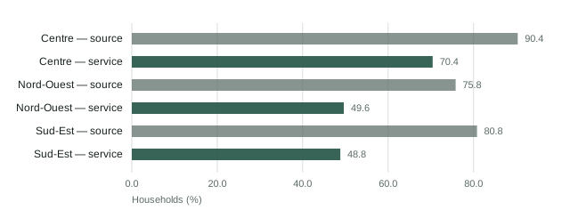
Both bars in each pair come from the same groupby. The only difference is which rows the numerator counts — and it moves the answer by twenty to thirty points in every district. That is what “the denominator is the point” means in practice.

Missing group keys are dropped

d = pd.DataFrame({"g": ["a", None, "a"], "v": [1, 2, 3]})

d.groupby("g")["v"].sum()                  # {'a': 4}
d.groupby("g", dropna=False)["v"].sum()    # {'a': 4, nan: 2}

By default groupby discards rows whose group key is missing. They vanish from the table and from the total, so the parts no longer sum to the whole and nothing says why.

In this sector the missing key is usually the interesting one: a facility with no district recorded, a household with no site code, a child with no commune. Use dropna=False and decide deliberately, or assert the key is complete:

assert muac["commune"].notna().all(), "rows with no commune would be dropped"

Unobserved categories reappear as empty rows

If the group key is categorical, the default is now to return only observed categories:

c = pd.DataFrame({"k": pd.Categorical(["x", "y"], categories=["x", "y", "z"]),
                  "v": [1, 2]})

len(c.groupby("k", observed=True)["v"].sum())    # 2
len(c.groupby("k", observed=False)["v"].sum())   # 3 — includes an empty "z"

Both are right for different questions. Reporting on facilities that submitted data wants observed=True; reporting coverage against a list of facilities that should have submitted wants observed=False, because a facility with zero rows is the finding.

Pass it explicitly. The default changed between pandas versions, and a script that relies on it produces a different table on a colleague’s machine.

Grouping by more than one key

by_commune_month = (
    muac.assign(month=muac["screening_date"].dt.to_period("M"), gam=gam)
    .groupby(["commune", "month"], observed=True)
    .agg(measured=("muac_mm", "count"), gam_cases=("gam", "sum"))
)

The result has a MultiIndex. Two ways to work with it:

by_commune_month.loc["Gonaives"]                      # one commune, all months
by_commune_month.reset_index()                        # back to flat columns

reset_index() before writing to CSV, always — otherwise the index columns either disappear or arrive unnamed.

To turn the long result into the wide table a report wants:

wide = by_commune_month["gam_cases"].unstack("month", fill_value=0)

fill_value=0 is safe here because a commune-month with no cases genuinely had zero. It would be wrong for a rate, where the absence means “not computed”, not “zero percent” — a distinction worth checking every time you reach for it.

transform: a group statistic on every row

agg collapses; transform returns a value per original row. This is how you compare a row against its own group without a join:

muac["commune_mean"] = muac.groupby("commune")["muac_mm"].transform("mean")
muac["vs_commune"] = muac["muac_mm"] - muac["commune_mean"]

Useful for flagging a site whose measurements sit systematically away from the rest — which is exactly the check the SMART survey analysis project uses to find a team measuring 0.5 kg light.

apply, and why to avoid it

apply runs a Python function per group and is the slowest thing in pandas by a wide margin. It is also the most flexible, so it is what people reach for first.

# Works, but slow, and returns something whose shape depends on the function.
muac.groupby("commune").apply(lambda g: g["muac_mm"].mean(), include_groups=False)

Prefer a named aggregation. Reach for apply when the operation genuinely needs the whole group frame — a per-group regression, a per-group ranking with ties broken on a second column — and pass include_groups=False, which is now required to avoid the grouping columns being handed to your function.

Pivot tables read better for a report

pivot_table is groupby plus unstack with a friendlier signature:

pd.crosstab(muac["commune"], muac["outcome"])

pd.crosstab(
    muac["commune"], muac["outcome"],
    values=muac["muac_mm"], aggfunc="mean",
).round(1)

crosstab with normalize="index" gives row proportions, which is usually what a referral table should show. Keep the counts beside them: a 50% referral rate on four children is a different fact from 50% on four hundred, and only the count distinguishes them.

Writing the result out

OUTPUTS = PROJECT / "outputs" / "tables"
OUTPUTS.mkdir(parents=True, exist_ok=True)

by_commune.reset_index().to_csv(OUTPUTS / "gam_by_commune.csv", index=False)

index=False after reset_index() — otherwise you get an unnamed integer column that someone will later open in Excel and sort by.

For a table someone will read rather than compute on, write the definition with it:

definitions = pd.DataFrame([
    ("GAM", "MUAC < 125 mm or bilateral pitting oedema",
     "children with a MUAC measurement or a recorded oedema assessment"),
], columns=["indicator", "numerator", "denominator"])

definitions.to_csv(OUTPUTS / "definitions.csv", index=False)

A number and its definition travel together, or the monthly argument about the denominator starts again.

What comes next

The table aggregates correctly and both halves of every rate come from one operation. The next unit gets the last piece right — dates, ages and reporting periods, where an age in months decides which growth standard applies — and then wraps the whole thing in a script that runs on someone else’s machine.